Zero Curve Methodology

Zero Curve Methodology

Zero Curve Conventions

A number of interest rate derivative valuation functions in the software require the user to pass a zero curve as an argument. This is accomplished by passing two arrays -- an array of zero curve dates (Excel serial date numbers) and a second array of zero rates associated with these dates. The user is free to pass their own zero curve provided that they observe the input conventions used in the add-in functions.

These conventions are:

i) the first element of the zero curve date array must be the valuation date (e.g. today);

ii) the array of zero curve dates must be in strictly ascending order;

iii) the array of annualized zero coupon rates are in continuously compounded form with a 365 day (fixed) year basis and in decimal form (e.g. six percent as 0.06); and

iv) the date and rate arrays must be of equal length (otherwise the software will truncate the longer array) and not longer than 200 elements. A longer array limit can be provided upon request.

A utility function called Yconvert is provided (see Section X) to convert rates to continuous compounding from other compounding bases.

Sample spreadsheets which accompany the software demonstrate the "bootstrap" methodology for generating a set of zero coupon dates and rates from combinations of cash, BAX/Eurodollar futures, and bonds plus swap spreads. These spreadsheets are then used to price FRAs, swaps, caps and floors, and swaptions.

The generic dates that tend to be used in most swap valuation systems are:

· Overnight, 1 week, 2 weeks

· 1 month, 2 months, 3 months, 6 months, 1 year

· thereafter in ½ year increments, to at least 10 years

For each date, the discount factor (present value of $1) and a continuously compounded zero rate are calculated using the methodology below in the samples:

Zero Curve Technical Details

· we use cash BAs/LIBOR out to 3 months

· we interpolate from the futures strip from 3 months out to 1 year

· we use the benchmark bond + swap spread thereafter (2, 3, 4, 5, 7, 10 years)

· the 1.5 year par swap rate is linearly interpolated between the 2 year all-in rate and the semi-annual equivalent of the 1 year rate

· discount factors are bootstrapped to exact swap curve dates, allowing for unequal periods due to weekends and/or holidays

· continuously compounded zero rates are derived from discount factors at bootstrap dates

· rates at arbitrary dates are linearly interpolated (except for the Hull-White model functions, which are always cubic-spline interpolated)

Zero Curve Formulae

I. Cash BA/LIBOR discount factors:

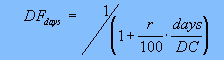
r = money market rate in percent form
days = actual days between valuation and maturity
DC = day count convention (actual 360 or 365)

II. Cash BA/LIBOR discount factors are converted to continuous compounded zero rates:

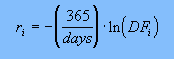
III. Cash BA/LIBOR rate at the nearest futures contract date is linearly interpolated from the continuous rates computed in II above. The discount factor at this date is then computed using:

IV. Discount factors out along the futures strip are computed recursively using:

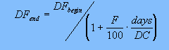
DF_end = discount factor at the end of the contract in question
DF_begin = discount factor at the beginning of the contract
F = forward rate implied in the futures price = (100 - futures price)
days = actual days covered by the futures contract

Continuously compounded zero rates are derived from these discount factors using the formula in II.

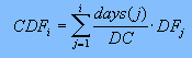
V. Discount factors out along the bond + swap spread strip (2 year + in Canada) are computed recursively to exact dates in half year increments using:

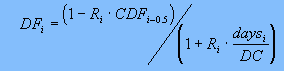
DF_i = discount factor at year i
R_i = par all-in swap rate at year i
CDF_i-0.5 = cumulative discount factor to the previous swap date

More details on zero curve construction can be obtained from published articles by David Smith (see Technical References).